Introduction
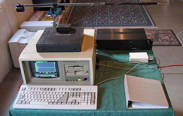
Here's my first-generation MLSSA system, still giving good results after 16 years. Behind the 486/33 computer, you can see the counterweighted low-diffraction mike stand (custom built by Mike Spurlock) fitted with a ACO Pacific 7012 1/2" instrumentation microphone. The Audionics CC-2 amplifier (to the right) powers the speaker under test, the little white box is a calibrated 20dB preamp, and the mike signal returns to the MLSSA card on the right side of the PC.
Although MLSSA is plenty fast at 160k/samples, the first-generation board I have has the disadvantage it only operates correctly in an 8MHz ISA slot. (The latest MLSSA 2000 still requires an ISA slot, but the new boards now work in a 16MHz bus. I've been waiting for a PCI version for some time now.) The EGA-display computer is on its 2nd motherboard and third hard disk, and seems to be holding up fine - of course, I only use it for the occasional MLSSA measurement, so it sees very light use.
It certainly has an interesting retro feel to start up the PC in DOS 6.0, note the April 6th, 1990 date of the original CELEST.TIM measurement, do a little post-processing to get the FRQ and WTR displays, save them as PCX files, copy them to a floppy, and take the floppy to a Dual G5 Macintosh running OS 10.4.7 and Photoshop CS at 2.7GHz.
(What? Install a ISA network card in a 486/33 PC running DOS? No thanks! Putting the disk into a USB-powered floppy drive is easier. I also have a modern AMD Athlon 64 X2 PC with a M-Audio Audiophile 192 PCI sound card, but there's something about the MLSSA software that's more intuitive and easier to use than general-purpose Windows XP audio programs. The best of all worlds would be MLSSA software that used industry-standard ASIO drivers to speak to 192/24 soundcards.)
This shows the time response of a Celestion SL-6 and the reflection off the floor (the small bump at 7.5 mSec). If the time window is large enough to include the floor bounce, when you do a FFT to see the frequency response, you get the comb spectra that appears in the green trace in picture below. If the time window is decreased to remove the floor bounce, the measurement window is about 2.5mSec long, and the frequency resolution is considerably degraded (the dotted yellow trace).
What to do? Neither corresponds to what you hear - for the interesting reason that the floor reflection actually assists in localization and the natural perception of timbre. (The BBC did a series of experiments of listening to stereo in an anechoic chamber, and found to their surprise that adding a plywood "floor" panel between the speakers and auditioner improved localization and gave a substantially more natural sound quality.)
Since the ear/brain/mind expects the reflection to be there, it's absence is perceived as unnatural - about the only time you don't hear a ground reflection is when you're on the balcony of a tall building, or sitting in a tree. The absence of a ground reflection signals "sitting very high" to the listener, which the ear/brain interprets as subtly threatening and unnatural.
But the floor bounce plainly isn't helping our measurements - MLSSA, and other measuring systems, aren't as thoughtful as an listener. If the MLSSA *.TIM files were easier to edit, I'd go in and clip the reflection out, joining the two sections together with a straight-line approximation.
Rather than hassle with editing files, I take the direct approach and use a 2-foot pile of assorted cushions where the floor bounce reflects off the floor; this reduces the floor reflection about 20dB, making it less troublesome for the subsequent FFT and waterfall calculations. (The feeble two inches of foam commonly seen in speaker cabinets has pretty feeble absorption capabilities, definitely not good enough for measurement work.)
The floor reflection has some interesting properties; with MLSSA or other MLS systems, you can look at the spectrum of the floor bounce by itself. What I've seen is the floor bounce is in the same phase as the direct sound, and the carpet rolls off high above 8kHz. Since the floor bounce is well off the vertical axis, the time and frequency response of the speaker can look a little distorted - although with the Celestion shown here, the similarity between the direct sound and the reflection is pretty obvious.
Some of the measurements in this series were made at home, and others at hi-fi shops. The travelling measurements don't have any floor bounce absorber, so the frequency data in some of these graphs look a little rough.
This is the time response of the Ariel, designed in 1993-1994. The crossover is an acoustic 4th-order, and so displays an initial rising pulse, a sweep downwards, and a return to the positive direction. This up-down-and-return is characteristic of all 4th-order crossover loudspeakers - well, I should correct myself: it's characteristic of 4th-order speakers that are two-way systems. A three-way system would have an additional up-and-down swing, but spread out over a much longer time span.
The smaller wiggles are driver artifacts, and the distinct small ripple at 420 microseconds appears to be some kind of reflection, either off the top of the cabinet or an internal reflection inside the cabinet. MLS is useful for finding these small reflections and letting you know if cabinet or driver modifications are working.
The final version of the Ariel you see here isn't as flat as the first attempts, which were extremely flat at plus or minus 1dB. Unfortunately they sounded pretty much like most other home-theater speakers with MTM driver layouts, forward and aggressive in the midrange. My guess is this is due to the narrowing vertical directivity of the MTM driver layout, which makes on-axis and total power-into-the-room frequency responses diverge.
After working on 13 crossover variations over six months, it became apparent that subjective flatness - which is more important than on-axis measurements - would require acceptance of a 1dB dip in the 3 to 4 kHz region, along with the original design goal of an overall 2dB tilt from 100 Hz to 10kHz (the woofers are 92dB efficient, the tweeter with no attenuation is 90dB). Subjectively, though, it sounds flat on pink-noise, and measures flat with 1/3 octave pink-noise measurements (which measure total power into a sphere, not just forward radiation).
Since the ear independently evaluates the direct-arrival spectra and compares it to the sum of the reflected spectra over the first 20 milliseconds, variations between the two are audible as colorations. This forces the designer to make a difficult choice between the direct-arrival on-axis measurement (seen here), a summation of many off-axis measurements (typically over a 60-degree frontal arc), and the total power radiated into the room (power radiated into a sphere).
Unless the speaker is an ideal omnidirectional radiator, these frequency-response measurements will depart from each other, and it is a matter of long-standing controversy which set of measurements correlate best with what you hear. (Anyone that tells you these things are not controversial is already a member of one of these camps, and has chosen to ignore other points of view.)
The Group Delay curve shows the apparent source location versus frequency - it's a fairly coarse scale at 1mSec/div, so one division corresponds to an acoustic distance of 14 inches. This shows another departure from the ideal point-source radiator, as the apparent source moves back and forth with changes in frequency. With well-behaved drivers and conventional crossovers, there's not much to see - with drivers in breakup and radical ultrahigh slope crossovers, though, some odd things start to appear.
I should mention here that MLSSA is not set to its standard defaults; I've changed the sampling rate to 102kHz, set the user-adjustable lowpass/anti-aliasing filters to 25 kHz with Bessel-filter slopes, set the window apodizing function to Blackman-Harris, and turned all frequency-smoothing display-filtering OFF. The 1/3 octave smoothing commonly seen in driver-manufacturer data sheets has not been used for any of the data shown in this article.
The high sampling rate combined with linear-phase lowpass filters avoids the impulse-response artifacts seen with many sound cards with brickwall filters at 20 kHz - by the way, quite a few 96/24 sound cards have fixed, non-adjustable 20 kHz brickwall filters, making them useless above 20 kHz. If you use a sound card to measure loudspeakers, I'd recommend the fastest one you can get, and make sure the the internal brickwall filter is 90 kHz or higher; I recommend a M-Audio Audiophile 192 sound card.
Between the 102 kHz MLS sample rate, 25 kHz Bessel lowpass filter, and the 7102 ACO Pacific microphone that goes out to 40 kHz, the measurements shown here are an accurate representation of the HF impulse response of these speakers. (Measuring ribbons with their 100 kHz response would be another story, requiring a lot more exotic equipment than I have now.)
In some quarters, it's matter of controversy whether to use cumulative-decay (waterfall) graphs at all. I find them quite useful for detecting narrowband resonances which don't appear on the conventional FR graphs shown above. We can see there are artifacts in the 1 to 3 kHz region - the slanted character points to crossover phase rotation, which we expect, and possibly the reflection that appears in the time-domain graph at the top. Reflections more serious than the one shown above, like a floor bounce, can completely disrupt the waterfall graph with clutter, and make it unreadable.
This is the other reason I absorb the floor bounce with a 2-foot pillow pile. I want to know what the drivers and cabinet are doing, instead of pretending resonances don't exist, and aren't audible. They may not be audible to a magazine reviewer, but I've been listening to crummy drivers since 1975, and don't care for the sound of driver resonances. If MLS can track down these resonances, I'll use it.
We can also see a group of narrowband resonances from 2.6 kHz to 10 kHz. One or two come from the Vifa midrange, but most are from the Scan-Speak tweeter; although they're not that pretty, as we will see in the other MLSSA data to follow, this is actually pretty good. In terms of audibility, the artifacts from 2.6 to 4 kHz are probably the most important.
Text and Pictures © Lynn Olson 2006.